BACKGROUND
COAs were originally developed for the 2006 State Wildlife Action Plan (SWAP), using the best available information at the time and with the intention to reassess boundaries with each revision of the SWAP to incorporate updated information. ODFW re-analyzed COA boundaries for the 2016 SWAP and again for the 2026 SWAP, using new and updated science, data, and resources.
MARXAN ANALYSIS
Marxan is a planning tool that identifies conservation areas using a cost-benefit analysis, optimizing for conservation goals (targets) while minimizing detrimental environmental factors (costs). The output from Marxan is a selection of individual conservation area units based on their cost value relative to the overall targets for the whole region. The analysis runs on a grid scale (planning units), and Marxan allows for individual planning units to be manually seeded at the beginning of the analysis or locked in/out of the final output. The 2026 revision used the same one square mile hexagon units that were used for the previous re-analysis in 2016.
Main Elements of Marxan Analysis
Costs
Costs were chosen for inclusion in the analysis based on potential or realized negative impacts to fish and wildlife species or their habitats. Other considerations for inclusion of information as cost factors included availability of spatial data to represent a specific cost, quality of available data, publication date (favoring newer data), and relevance to present-day conditions.
Cost factors used in the 2026 analysis included:
- Agricultural land presence
- Aquatic pollution
- Burn probability (annual)
- Burn severity of past fires
- Existing landscape protections (USGS GAP Status)
- Impervious surfaces (development)
- Observed presence of invasive species
- Mining operations (geographic footprint)
- Modeled data for detrimental climate change impacts
- Solar field presence
- Terrestrial pollution
- Wetland drying trends
Cost factor source data were translated to fit the hexagon grid by calculating the proportion of coverage of each factor within each one square mile hexagon unit. For each cost factor, a numerical weighting value was assigned to represent that factor’s impact on the landscape. Weight values were based on feedback from ODFW staff. All cost factors were compiled into a single cost value for each hexagon by multiplying each factor’s proportion of coverage by its weight and then taking the sum of all the weighted factors:
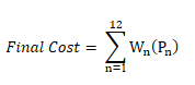
Where Pn is the proportion of coverage for the nth cost factor and Wn is the respective weight for that cost factor
Targets
Marxan targets were chosen for inclusion in the analysis based on potential or realized presence of Species of Greatest Conservation Need (SGCN) and Key Habitats. Targets were selected based on discussions with regional and local experts and included consideration of the targets used in 2016 analysis. Other considerations for inclusion of information as target factors included availability of data to represent a specific target, quality of available data, publication date (favoring newer data), and relevance to present-day conditions.
Target factors used in the 2026 analysis included:
- Modeled data for climate stability
- Environmental Justice Index (EJI)
- Key Habitat presence (based on the draft 2026 Key Habitat map)
- Intact connected habitats expected to support diffuse wildlife movement
- Observed presence for each SGCN
- Modeled range for each SGCN (USGS GAP Species Data)
Target source data were translated into the hexagon grid such that each target was considered separately (i.e., a single hexagon could have coverage for multiple, overlapping targets). Coverage was calculated based on the data type: for polygon and raster data the proportion of coverage was calculated, while for point data (SGCN presence) a binary presence/absence value was used to represent whether the species was observed anywhere within a given hexagon. The SGCN observation and range datasets and the Key Habitat datasets used for each ecoregion included only SGCN/Key Habitats designated for that ecoregion.
In total, the 2026 Marxan analysis included over 300 separate data layers statewide.
Calibrations
Ecoregion-specific targets and target goal values
For each target, a goal value was set representing the desired proportion of the target’s total presence in each ecoregion. These goals were based on the amount and distribution of each target across the landscape, factoring in target rarity and degree of endangerment to ensure that each target was treated equally. Targets should be represented in multiple COAs (where possible) as a hedge against stochastic events (e.g., disease, fire) and to buffer against the anticipated impacts of climate change, with an overarching intention to provide for long-term viability of SGCN and Key Habitats across the state.
Conservation target data sets were tailored to each ecoregion such that the SGCN observation datasets, SGCN range datasets, and the Key Habitat datasets used for an ecoregion included only those species or habitats designated as SGCN or Key Habitats for that ecoregion. Goal values were determined for each SGCN based on each species’ conservation status and distribution in Oregon, with more imperiled species and species with smaller distributions receiving higher goal values. These goal values help drive the selection of COAs. For example, if a species in a given ecoregion had a goal value of 20%, the Marxan output (the full set of chosen hexagon units) would be required to include at least 20% of that species’ range within the chosen hexagons for that ecoregion. Goals for Key Habitats were generated using an overall range of 30 percent (the recommended minimum amount of habitat needed to sustain imperiled populations) to 60 percent (the recommended maximum amount of habitat to be included while still prioritizing distinct areas).
Boundary Length Modifier and Number of Iterations
The Boundary Length Modifier is used to determine the relationship of the size of conservation areas versus the number of distinct conservation areas (e.g., few large areas vs. many smaller areas). The Number of Iterations value represents the number of randomly selected comparisons that Marxan will make during each modeling run. Each ecoregion was calibrated separately for each of these values to optimize the results without compromising the total cost or data processing efficiency.
Refining Results
The Marxan analysis was run for each ecoregion independently.
The raw results were refined using an iterative process that considered several sources of additional information:
- Initial results were filtered to exclude GAP Status 1 areas. GAP Status 1 lands are areas managed for biodiversity where natural disturbances are allowed to proceed. In Oregon, GAP 1 lands include designated wilderness areas and Crater Lake National Park. These areas have permanent protection from conversion of natural land cover and on-the-ground habitat and restoration work is typically prohibited, so opportunities for the development of conservation projects is limited compared to other areas in the state.
- The 2026 initial Marxan results were overlaid with the 2016 initial Marxan results and overlapping hexagons were flagged for automatic inclusion in the draft 2026 COA boundaries for reviewer feedback. Hexagons selected in two separate analyses undertaken ten years apart are likely indicative of areas with consistently high conservation value.
- The final 2016 COA boundaries were overlaid with the initial Marxan results from 2016 and 2026. Hexagons from the 2016 COA boundaries that did NOT overlap with the initial Marxan output from either the 2016 or the 2026 analyses were flagged for automatic exclusion from the draft 2026 COA boundaries for reviewer feedback. Hexagons selected in neither of two separate analyses undertaken ten years apart are likely indicative of areas with consistently low conservation value.
- The results of modeling and refinement process were compiled into draft boundaries for internal and external review. Draft 2026 COA boundaries were adjusted using feedback from two separate review periods in April and again in May/June of 2025 to produce final COA boundaries for the 2026 SWAP. All feedback that was relevant to COA boundaries was evaluated and specific hexagons that were highlighted were considered for edits to COA boundaries. In cases where reviewers provided detailed, local knowledge of landscape suitability for SGCN or other factors that ran counter to the results of the modeling and refinement process, the reviewer feedback took precedence.
After selecting hexagons to include in the final product, boundary lines were then drawn to delineate distinct COAs. All 2026 COA boundaries were clipped to the Oregon state boundary.